Neural Ordinary Differential Equations

Neural Ordinary Differential Equations (Neural ODEs) [1] surfaced in 2018 as a computationally tractable model for the training of neural networks without a specification of the number of layers also known as depth. Neural ODEs describes a model that learns the derivative, $f$, of a target function $z$ where the depth of the model network is unknown. The implied similarity with ordinary differential equations is expressed in its output being obtained through integration over the network.

The computational efficiency of the model offers impressive training and evaluation/classification execution-time. Since the publication of this paper, describing the model, improvements have been suggested [2] to overcome failures of NerualODEs for certain benchmark problems. Neural ODEs may fail to accurately model the dynamics for some classes of benchmark problems. The paper further explores two applications of Neural ODEs: continuous time-series models and invertible normalizing flows.

This article focuses on describing the elements and methods used by Neural ODEs and how these models can be trained. The goal is to study how the dynamics of a target function can be learnt in a supervised learning setting. It is assumed that the reader is somewhat familiar with neural networks and related terminology.

In this article:

• Principles of Neural ODEs
• Model Evaluation
• Model Training

Neural Ordinary Differential Equations for supervised learning

Neural Ordinary Differential Equations are a new type of neural network models that learns the dynamics of a target function $z$. Where neural networks are described by interconnected layers, a Neural ODE is computed using integral:

$$ z(x,t) = z(x,t_0) + \int f(x, \theta, t) dt $$

. Where $f$ models the dynamics, $x$ is the output of the previous integral (the input at initiation), $\theta$ are the hyper-parameters (neural weights etc.) and $t$ is the variable of integration. Although the variable of integration, $t$, resembles depth, it should be noted that different initial values of the input potentially leads to different step lengths during integration. This notion of depth is unlike standard models which explicitly state the number of interconnected layers. For now, this is simply an observation and in the remainder of this article $t$ is referred to as the depth without further consideration.

Let the dynamics, $f$, be modelled by the (possibly) recursive neural network layer with weights $\theta$:

$$ f(x, \sigma) \approx \sigma(x, \theta, t) = \sigma_{n}(\sigma _{n-1}, \theta, t_n) $$.

Here it is highlighted that the output of a layer $\sigma_{n-1}$ is the input to the subsequent layer $\sigma_n$. The difference in depth, $(t_n - t _{n-1}) = \Delta t_n$ is determined by some constraint of the error for example. Depending on the numerical integration scheme, $\Delta t$ can be therefore be constant or variable (adaptive).

With a trained neural ODE, computing $\hat{z}(t)$ means feeding the input through the neural model in a forward pass. When evaluating the Neural ODE model, the output is computed using a numerical integration scheme $\hat{\int}$: $$ z \approx \hat{z}(t, x) = z(x, t_0) + \hat{\int _{t_0}^{T}}f(x, \sigma, t) dt $$ with initial depth $t_0$ and maximum depth $T$.

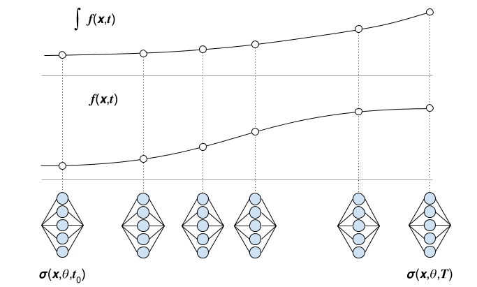
Figure: Illustrating evaluations of the Neural ODE ($\sigma$) and the target function ($z$).

During training, the evaluations of $\sigma$ are tracked in order to (back)propagate derivatives. Training involves computing the loss $\mathcal{L}(y,\hat{y})$ and applying the gradient update to $\theta$:

$$ \theta _{n+1} = \theta_n + \lambda \dfrac{\partial \mathcal{L}}{\partial \theta}, $$

where $\lambda$ is the learning rate.

Numerical integration

Computationally approximating a primitive function at some sought value can be performed reliably using a numerical integration scheme. There are various types of schemes that have different computational cost, numerical accuracy and stability. The most straightforward such method is Euler’s method of integration which states that: $$ y(t + \Delta t) \approx y(t) + \Delta t f(t), $$

where $y(t)$ is some known state of the primitive function, $f(t)$ is its derivative and $\Delta t$ is some step size. Euler’s method lacks sufficient accuracy and stability to be reliably employed for the application of Neural ODEs. There exist methods, such as the family of Runge-Kutta methods that provide higher accuracy and stability, allowing for fine control of the error tolerance.

Forward pass - Evaluation/Classification

The Neural ODE is evaluated by passing the input $x$ to the Neural ODE model or layer. Computing $z(t)$ means integrating $\sigma$:

$$ \hat{z}(x,t) = z(x, t^{*}, \theta^{*}) + \int _{t_0}^{t} \sigma(x, \theta^{*}, t^{*}); dt $$

where superscript $^{*}$ is taken to mean optimized (learnt) from initial guess $t^{0},\theta^{0}$. Provided that $\sigma$ is an accurate estimator of $f$, $\hat{z}(t)$ can be computed to arbitrary accuracy using a carefully selected numerical integrator.

Backward pass - Training

The goal of training is to update the model parameters $\theta$. As a measure of error, a loss-function $\mathcal{L}$ is set. One such example is the mean squared error $\mathcal{L} = || z - \hat{z} ||^2$. The loss function computes the difference between the target ($z$) and the estimation ($\hat{z}$). The rate of change of the loss with respect to $\theta$ (denoted $\mathcal{L}_{\theta})$, is a vector pointing toward increasing loss (positive gradient). Taking the negative gradient points in the direction of decreasing loss. This direction is used to guide an update to $\theta$ which, supposedly, minimizes the loss. These gradients are computed during backpropagation, using a reverse-mode differentiation technique called the adjoint method to efficiently compute all required derivatives. This technique consists in computing the derivatives from the final value of the loss function and propagating them through the neural layers $f(f(f( \cdots (x,\theta))))$ in reverse order. “Efficiently”, is this case refers to obtaining a smaller system of equations than developing derivatives starting from the input [3].

Backpropagation for Neural ODEs

For convenience the function $z$ will from here on contain the parameter $t$ which represents a “depth-like” parametrization. In most cases, $z$ will not depend on $t$. Instead, $t$ quantifies the step length between evaluations of the dynamics.

The gradient of the loss with respect to $z$ is called the adjoint:

$$ a(t) = \dfrac{\partial \mathcal{L}}{\partial z(x, \theta, t)}. $$

Note that this partial derivative is conditioned on $\theta$ being fixed. In other words, this partial derivative evaluates the response to a small (infinitesimal) change in the value of $z$. Then, to compute derivates with respect to $\theta$:

$$ \mathcal{L}_{\theta} = \dfrac{d\mathcal{L}}{d\theta} = - \int _{T}^{t_0} a(t)\dfrac{\partial f(z,\theta,t)}{\partial \theta} dt $$

Note that the integral interval is from $[T,t_0]$ (reverse) and that the sign is flipped.

The partial derivative of the loss w.r.t. each evaluation of $z$ (the adjoint $a(t)$) can be computed and recorded during the forward pass, and in fact this is performed by neural network frameworks that support automatic differentiation. Having $\frac{da(t)}{dt}$ the authors propose to compute $a(t)$ by, yet again, computing the integral

$$ a(t) = - \int _{t_n}^{t _{n-1}} a(t)\dfrac{\partial f(z,\theta,t)}{dz} dt $$

Example: adjoint computation of dynamics $f$

To exemplify this, consider the simple dynamics function $f(z,\theta) = Wz$ where $W$ is a matrix with elements equal to the parameters of $\theta$. Each gradient with respect to $z$ and $\theta$ is described below.

Gradient with respect to layer depth

$$ \begin{eqnarray} \dfrac{\partial a(t)}{\partial z(t_0)} &=& - a(t)\dfrac{\partial f(z, \theta, t)}{\partial z(t)} \\\ &=& - a(t)\dfrac{\partial W z(t)}{\partial z(t)} \\\ &=& - a(t)W \end{eqnarray} $$

thus, the sought value can be found by numerically integrating $-a(t)W$.

Gradient with respect to weights

Recall that $W$ consists of the elements of $\theta$:

$$ \begin{eqnarray} \dfrac{\partial a(t)}{\partial \theta} &=& - a(t)\dfrac{\partial f(z, \theta, t)}{\partial \theta} \\\ &=& - a(t)\dfrac{\partial W z(t)}{\partial \theta} \\\ &=& - a(t)z(t) \end{eqnarray} $$

References

1. Chen R. T. Q, Rubanova Y., Bettencourt J, Duvenaud D. 2019. Neural Ordinary Differential Equations. arXiv:1806.07366 (cs.LG)
2. Dupont E., Doucet A, Yee Whye T. Augmented Neural ODEs arxiv.org:1904.01681 (stat.ML)
3. G. Johnson. S. Notes on Adjoint Methods for 18.335. PDF