One-shot training Neural Networks using geometric bounds

Machine learning, in particular the class of neural networks, has propelled classifying and prediction type tasks into what is today the state-of-art in many fields. Compared with other approaches, neural networks display an outstanding ability to learn from examples. In order to harness the predictive and classifying capabilities of neural networks a great amount of training data must be prepared and fed through the network. The sheer amount of data required often becomes large. The huge amount of data in combination with high computational effort during training makes standard PC and server processors infeasible for the task. To combat the ever growing amount of required processing power machine learning developers and researches recruit the help of co-processors such as GPUs and other custom hardware to train and evaluate the neural nets.

Not only is the time to train networks burdening, the cost of purchasing and operating large and complex clusters is considerable. To this end, increasing the learning speed of neural networks results in massive resource savings in both invested time and operational costs especially considered at corporate scales.

This article presents the method and recreates the results of a recent (2019) paper called “A Constructive Approach for One-Shot Training of Neural Networks Using Hypercube-Based Topological Coverings” [1]. It presents a method of inferring the parameters (weights and biases) and structure of a neural network from linear bounds. Effectively replacing the traning step with an (cheaper) analysis step from which the final (ready trained) network is set.

In this article:

• Breakdown of the linear bounds feature space discretization
• Mapping linear bounds to neural network parameters
• Test results on Iris dataset

Linear bound discretization

The feature space of a dataset can have any dimension ranging from small datasets with low dimensionality, like the Iris dataset [2], to large high-dimensional datasets like ImageNet. The paper [1] introduce a constructive method for covering the feature space of the dataset with geometric covering maps. A map consists of a lower and upper boundary in each dimension that enclose a space containing samples from the same (homogeneous) or different (inhomogeneous) class of samples. There also exist maps that span empty spaces in order to provide a total covering of the feature space. The animation below shows two homogeneous hypercubes in $N = 3$

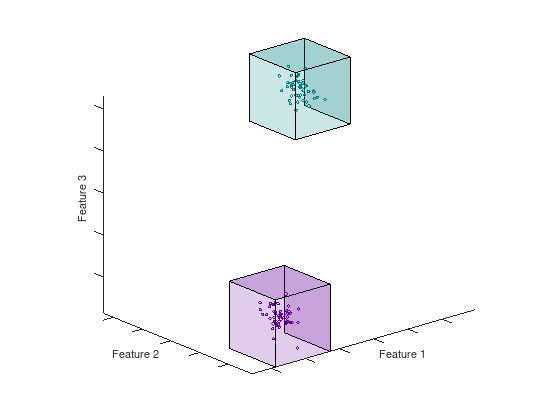
Figure: Hypercubes in 3D are box volumes defined by their bounds in each dimension.

These maps corresponds to a set of linear inequalities associated with each class as well as its homogeneous and inhomogeneous state. For example, a map ($H$) covering some region of a $N = 2$ dimensional space would be

$$ H = \lbrace B , S \rbrace \ $$ where $B$ are the bounds in each dimension and $S$ is the state of the points enclosed by the bounds: $$ B = \lbrace (b_1^<, b_1^>) , (b_2^<, b_2^>) \rbrace $$ $$ S \in \lbrace Inhomogeneous, Homogeneous, Empty \rbrace $$

The maps $H$ are called hypercubes in the paper. The state of a hypercube is determine by whether it enclose zero ($Empty$ or simply $H_E$), equal ($Homogeneous$ or simply $H_H$) or mixed ($Inhomogeneous$ or simply $H_I$) sample classes. The following example illustrates how a sample is evaluated if it is enclosed in a specific hypercube or not.

Example 1: Evaluating if a sample is inside or outside a hypercube

Let the input sample $x$ consists of the features vector $x = [3.2, 0.7]$ and consider the hypercube $H$ having bounds $\lbrace (0.1, 2.7), (0.0, 1.2) \rbrace $. If the sample is inside $H$ all feature values of $x$ must be within the corresponding bounds. Since the first feature value is outside the bounds $$b_1^{<} \leq b_1^{>} \leq x = 0.1 \leq 2.7 \leq 3.2$$ and although the second feature is inside the bounds $$b_2^{<} < x_2 < b_2^{>} = 0.0 \leq 0.7 \leq 1.2$$ the sample is outside of $H$.

By computing the boundaries of hypercubes such that they optimize for homogeneity, a total covering of any feature space can be calculated. The total feature space is thus composed of a set of empty, homogeneous and inhomogeneous hypercubes.

Bisecting the feature space with hypercubes

Consider a dataset that contains samples (feature vector $x$) and a class label $c \in C$. The approach described in the paper is initiated by a (inhomogeneous) bounding box (hypercube) over the entire dataset and is iteratively bisected into progressively homogeneous non-overlapping hypercubes. Bisection is not allowed if any of the resulting bounds is shorter than a minimum length scale $l$. Further more, bisection is also constrained on the aspect ratio of the shortest and largest bound $r^{*} \leq \frac{min(B)}{max(B)}$. These simultaneous constraints ensure that the bisection does not result in overfitting.

Bisection is continued until either there are no more inhomogeneous hypercubes or bisection would violate the minimum length constraint or the aspect ratio constraint. The following pseudo-code exemplifies the overall procedure:

H_H = []
H_E = []
H_I = [boundingBox]

while not empty(H_I):
  H = pop(H_I)

  # Symbols in [1]:                     l                   r*
  H_a, H_b = bisect(H, dataset, minLengthConstraint, aspectRatioConstraint)

  if empty(H_a) and empty(H_b): # bisection would violate l and r*
    return H_H

  addToClassSet(H_a, dataset, H_H, H_I, H_E)
  addToClassSet(H_b, dataset, H_H, H_I, H_E)

After having successfully bisected the feature space the resulting homogeneous hypercubes are translated into linear bounds which can be applied directly to weights and biases in neural networks as described in the next section.

The specifics of how bisection is performed subject to constraints $l$ and $r^{*}$ can be studied in the paper.

Mapping linear bounds to neural network parameters

The set of all bounds in (homogeneous) hypercubes $H_c$ that enclose features of class $c$ is able to classify samples strictly based on the training set. Furthermore, the hypercubes are unable to provide a meaningful classification of points in-between two hypercubes of different classes. Another way of describing this inability is to consider the binary outcome of testing whether a sample is inside the bounds of the hypercube or not. In order to classify samples based on its proximity to other hypercubes, the approach in [1] is to map the bounds of all hypercubes associated with each class into a neural network such that the output of such a network is a rectifying activation function (ReLU). This extension enables more complex delineations in the terms of the classes boundaries.

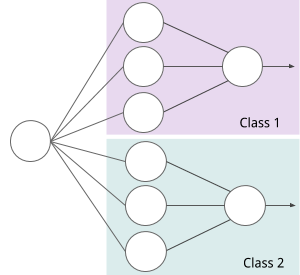
The structure of the neural network is constructed as a composition of smaller sub-networks. The input $x$ is connected to each sub-network. Each sub-network classifies a distinct class membership $c$. The output of each sub-network is a value $[0, 1]$ where $1$ is interpreted as full activation (class membership). The combined output of every sub-network is fed into the softmax function yielding a one-hot output as commonly applied by other types of neural networks.

A sub-network is translated from the bounds of hypercubes. That is, each sub-network is translated from a set of hypercubes $\lbrace H_c^1, H_c^2, … , H_c^i \rbrace ;, c \in C $ all enclosing a homogeneous feature space of class $c$. The figure below illustrates a structure created for two classes each having one hypercube with boundaries for three dimension ($N = 3$).

The linear bounds are translated into a rectifying activation using the following expression.

$$ f(x_n, b_n^<, b_n^>) = ReLU(-x_n + b_n^{<}) + ReLU( x_n - b_n^{>}) $$ where $ReLU(x) = max(0, x)$. Each activation $f_n$ is added to the sum $\Theta_k$. The following example provides some clarification

Example 2: Computing the sub-network output activation

Take again the example input and bounds from Example 1. Input $x$ consists of the features vector $x = [3.2, 0.7]$ and consider the single hypercube $H$ having bounds $\lbrace (0.1, 2.7), (0.0, 1.2) \rbrace $. The activation for the sample $x$ is then: $$ f_1(x_1, b_1^<, b_1^>) = ReLU(-3.2 + 0.1) + ReLU(3.2 - 2.7) = 0.0 + 0.5 $$ $$ f_2(x_2, b_2^<, b_2^>) = ReLU(-0.7 + 0.0) + ReLU(0.7 - 1.2) = 0.0 + 0.0 $$ and finally $\Theta_k(x) = f_1 + f_2 = 0.5$.

Similarly for another sample $x_2 = [0.5, 0.5] $that is inside $H$: $$ f_1(x_1, b_1^<, b_1^>) = ReLU(-0.5 + 0.1) + ReLU(0.5 - 2.7) = 0.0 + 0.0 $$ $$ f_2(x_2, b_2^<, b_2^>) = ReLU(-0.5 + 0.0) + ReLU(0.5 - 1.2) = 0.0 + 0.0 $$ and finally $\Theta_k(x_2) = f_1 + f_2 = 0.0$.

The structure of the sub-network is illustrated in the figure below

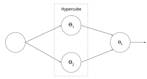
Neural network translation

For a given hypercube $H_k$, the boundaries $b_n^<$ and $b_n^>$ are translated into the corresponding matrix system of weights $W_k$ and biases $v_k$

$$ W_k x + v_k \leq 0 $$

. This formulation is represented by a hidden neural network layer. The weight matrix $W_k$ and bias $v_k$ of the layer is

. $ReLU(\cdot)$ is applied element wise to the result of $W_kx + v_k$ and gets added to the sum $\Theta_k$. At this point the output is zero to indicate class membership and a positive value else. To invert the output, a simple modification can be applied

$$ 1 - min(1, \Theta_k)$$

which fully describes the translation from linear bounds into a neural networks for a class $c$.

Classification results

These results are compiled by taking the average prediction accuracy over 20 runs. The results are run on the Iris [2] and Wine [3] datasets. Data is split into 70% training and 30% testing sets. The runtime is heavily influenced by the choices of $l$. For example, it is observed that the runtime takes between 2ms to 30ms depending on $l$ resulting in a variation in accuracy of 5-10%. The implementation was made in the Rust programming language.

+--------+----------+---------+
|Dataset | Accuracy | Std.dev |
+--------+----------+---------+
| Iris   |  94.5%   |  3.3%   |
| Wine   |  75.4%   |  7.5%   |
+--------+----------+---------+
|     Results from paper      |
+--------+----------+---------+
| Iris   |   96%    |  2.3%   |
| Wine   |   87%    |  4.4%   |
+--------+----------+---------+

Note that the both the Iris and Wine dataset are classified without preprocessing the data. In the paper it is stated that both the Iris and Wine dataset by using PCA before performing bisection. The results are thus not directly comparable but similar enough to be presented side-by-side in this setting.

Acknowledgement

This project was co-developed with a friend and former colleague who goes by the nickname Okunnig.

References

1. W. Brent Daniel, Enoch Yeung 2019. A Constructive Approach for One-Shot Training of Neural Networks Using Hypercube-Based Topological Coverings arXiv:1901.02878 (cs.LG)
2. Iris dataset: https://archive.ics.uci.edu/ml/datasets/iris
3. Wine dataset: https://archive.ics.uci.edu/ml/datasets/wine

Found an error? Report it by email and I will put your name and contribution in the article.