Fast signal parameter estimation and reconstruction using autoencoder
August 20, 2021The paper Rapid parameter estimation of discrete decaying signals using autoencoder networks [1] demonstrates the usage of machine learning models for fast$^1$ parameter extraction in signals of the form:
$$ \begin{eqnarray} y_{\textrm{exp}} &=& A_0\cdot e^{-t/\tau} + y_0 \\\ y_{\textrm{osc}} &=& A_0\cdot e^{-t/\tau} \cdot cos(2\pi \cdot f \cdot t + \phi) + y_0 \end{eqnarray} $$
That is, the model estimates parameters of these two types of signals. The parameters govern the steepness, amplitude, frequency and noise of both signals. Each type of signal is shown in the examples below:
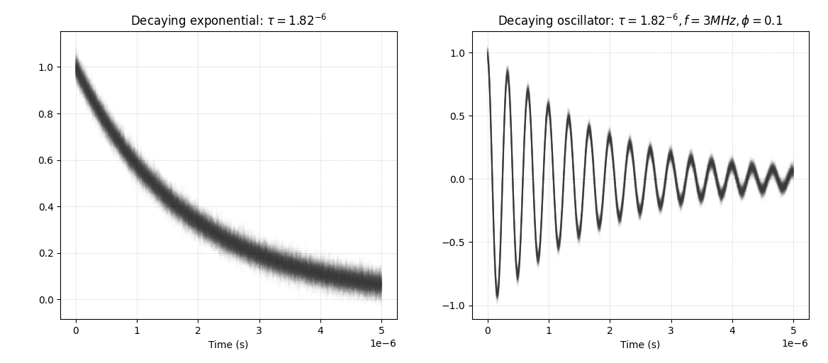
Figure: Example of 100 decaying exponential (left) and oscillator (right) signals with random noise $y_0$.
These benchmark signals represent a typical use case in many scientific instruments for example Nuclear Magnetic Resonance and Cavity Ring-Down Polarimetry/Ellipsometry (CRDP/CRDE) [1] to analyse the chemical constituents of substances. The signals typically have fast decay times in the order of $[10^{-2}, 10^{-1}]$ in case of NMR and $[10^{-7}, 10^{-5}]$ in CRDP/CRDE. These fast decay times pose a challenge for instruments which struggle to estimates paremeters at speeds up to 4.4kHz, even when implementing specialized hardware using frequency-based methods.
The goal of the method described in the paper is to achieve higher rates of analysis using autoencoder machine learning methods. The autoencoder model is fed a signal as input and recovers estimated parameters $\tau, f, \phi$. The results demonstrates the high efficiency of model which manages to recover parameters at much higher rates (200kHz) even while running on non-specialiced commodity hardware. The goal of this article is to reverse the model and train such an autoencoder model to estimate parameters as outlined in the paper.
In this article:
- Autoencoders implemented using dense neural network layers
- Model training and evaluation
Dense neural network autoencoder layers
An autoencoder is a machine-learning model that learns latent data encodings. An autoencoder is composed of an encoder model that compress input to a latent representation and a decoder that reconstruct input from the that latent representation. Given input $X$ the autoencoder will output $f(X) = \hat{X}$ which should reconstruct $X$ as well possible. The architecture of the autoencoder is such that it maps inputs $X$ to a latent representation $z \in L$. The dimensionality of $L$ is a design parameter. This part is usually thought of as a compressing step as the latent space can be smaller than $X$ (although larger spaces exist too). The last part is the decompressing part which reconstruct $X$ from a sample $z$ in the latent space. The entire autoencoder is sometimes depicted as below:
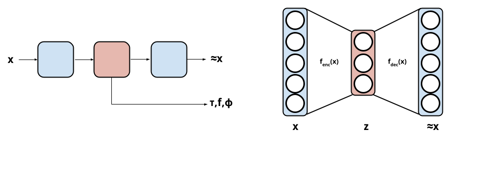
Figure: Left: box-model depiction the autoencoder interface. Right: model depiction of the autoencoder network.
The autoencoder in the paper uses dense neural network layers that are symmetric in both the encoder and decoder. In this work the latent space have the same number of dimensions as the number of parameters sought to be learnt. The number of neurons in each layer, in case of the decaying exponential, is $1000, 50, 1, 50, 1000$ and $1000, 50, 10, 3, 10, 50, 1000$ in case of the decaying oscillator. The number of layers and their width was determined experimentally according to the paper and moreover the neural activation function is the hyperbolic tangent.
Training
Training is performed in three-steps:
- Train the whole autoencoder.
- Train the encoder part separately.
- Train the decoder part separately.
These steps are repeated 10 times for a dataset containing samples from $y_{\textrm{exp}/\textrm{osc}}$ having fixed $\tau, f, \phi$ and noise $y_0$. In total the autoencoder is trained on 10 such datasets with an signal-to-noise ratio of $2^{20}$.
The three-step method enforce both that parameter extraction from the latent representation is meaningful and that this representation matches the parameters of interest (and not something else). The authors show experimentally that this three-step training converge to the same result as training the whole autoencoder only, while satisfying both requirements for parameter extraction and signal reconstruction.
The three-step training is repeated for 10 different choices of $\tau, f$ and $\phi$. In creating the signals, the following distributions are used:
$$ \begin{eqnarray} \tau &\sim& ||N(1\mu s, 0.5\mu s)|| \\\ f &\sim& N(3 \textrm{MHz}, 0.1 \textrm{MHz}) \\\ \phi &\sim& N(0, 0.1) \end{eqnarray} $$
The encoder output for estimation of $\tau$ (exponential decay) is shown below after training on each of the ten databases:
Results
Using the above training paradigm to learn an encoder to estimate $\tau$ the result from such an estimation is compared side-by-side with a numerical least-square fit of the parameter. The figure below was created using a model built and trained using Tensorflow.
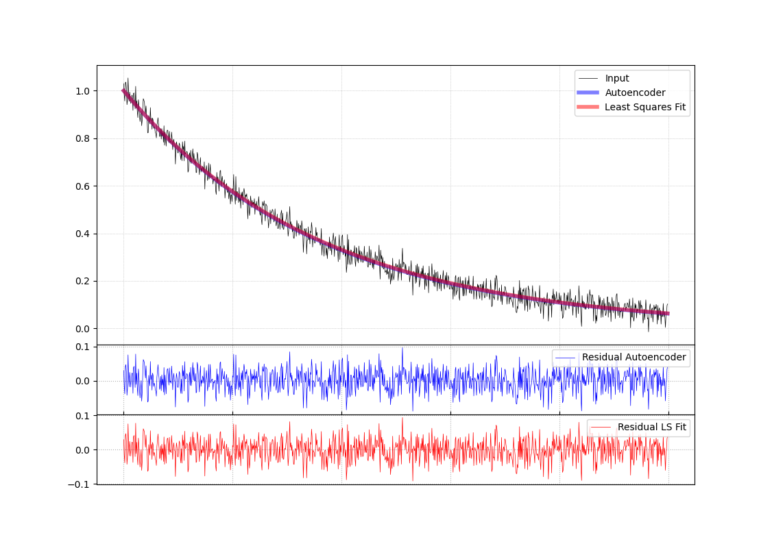
Figure: Reconstructed results from Figure 4a in the paper: Reconstructed signal during 5$\mu$s using autoencoder (blue)
compared to least squares fitted model (red)
References
- Visschers J, Budker D., Bougas L. Rapid parameter estimation of discrete decaying signals using autoencoder networks arxiv.org:2103.08663 (eess.SP)